Dynamic-VINS
关于论文 RGB-D Inertial Odometry for a Resource-Restricted Robot in Dynamic Environments (RA-L, 2022) 的阅读总结。
Information
- Title: RGB-D Inertial Odometry for a Resource-Restricted Robot in Dynamic Environments
- Authors: Jianheng Liu, Xuanfu Li, Yueqian Liu, Haoyao Chen
- Conference: RA-L, 2022
- Source Codes: https://github.com/HITSZ-NRSL/Dynamic-VINS
1 Introduction
Problems with visual SLAM:
- Most existing vSLAM systems rely on static environment assumptions, and stable features in the environment are used as solid constraints for Bundle Adjustment.
- In real scenarios, dynamic objects may adversely affect pose optimization. Although RANSAC and other methods can suppress the influence of dynamic features to some extent, when a large number of dynamic objects appear in the scene, it makes these methods difficult to use.
Some solutions and their limits:
- Pure geometric methods
- Limits: unable to cope with latent or lightly moving objects.
- Deep learning based
- Methods: exploiting the advantages of pixel-wise semantic segmentation for a better recognition of dynamic features.
- Limits: expensive computing resource consumption of semantic segmentation.
- Semantic segmentation on keyframes
- Methods: performing semantic segmentation only on keyframes and track moving objects via moving probability propagation.
- Limits: since semantic segmentation is performed after keyframe selection, real-time precise pose estimation is inaccessible, and unstable dynamic features in the original frame may also cause redundant keyframe creation and unnecessary computation.
The above systems still require too many computing resources to perform robust real-time localization in dynamic environments for Size, Weight, and Power (SWaP) restricted mobile robots or devices.
Some embedded computing platforms are euqipped with NPU/GPU computing units, which enable lightweight deep learning networks to run on these platforms. However, it is still difficult to balance efficiency and accuracy for mobile robot applications.
This paper proposes a real-time RGB-D inertial odometry for resource-restricted robots in dynamic environment named Dynamic-VINS. The main contributions are as follows:
- An efficient optimization-based RGB-D inertial odometry is proposed for resource-restricted robots in dynamic environments.
- Dynamic feature recognition modules combining object detection and depth information are proposed.
2 System Overview

Dynamic-VINS is extended based on VINS-Mono and VINS-RGBD. Three main threads run parallel (Object detection, feature tracking, state optimization):
- Color images are passed to object detection and feature tracking;
- IMU measurements between two consecutive frames are preintegrated for feature tracking and state optimization.
Feature tracking thread: track features detected by grid-based feature detection with IMU preintegration.
Object detection thread: detect dynamic objects in real-time.
State optimization thread: summarize the features information, object detection results and depth image to recognize the dynamic features.
3 Methodology
- Semantic and geometry information from RGB-D images and IMU preintegration are applied for dynamic feature recoginition and moving consistency check.
- The missed detection compensation module plays a subsidiary role to object detection in case of missed detection.
- Dynamic features on unknown objects are further identified by moving consistency check.
3.1 Feature Matching
For each incoming image, the feature points are tracked using KLT sparse optical flow method, while IMU measurements between frames are used to predict the motion of features. Reducing optical flow pyramid layers provides better initial position estimation of features. Fig. 2 is the basic idea.
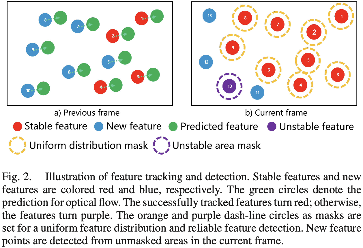
When the current frame arrives:
- IMU measurements between the current and previous frames are used to predict the feature position (green) in the current frame.
- Optical flow uses the predicted feature position as the initial position to look for a match feature in the current frame:
- Successfully tracked features are turned red;
- Features failed to be tracked are marked as unstable (purple).
- Masks (dash-line circles):
- Orange mask centered on the stable features are set to avoid the repetition and aggregation of feature detection.
- Purple mask centered on the unstable features are set to avoid unstable feature detection.
- New features (blue) are detected from unmasked areas in the current frame.
3.2 Grid-Based Feature Detection
System maintains a minimum number of features for stability, and features need to be extracted constantly.
Grid-based feature detection:
- Divide image into grids and pad the boundary of each grid to prevent the features at the edges of grids being ignored.
- Conduct feature detection on the grids with insufficient matched features.
- The grid cell that fails to detect features due to weak texture or is covered by the mask will be skipped in the next detection frame to avoid repeated useless detection.
- The thread pool technique is used to reduce time consumption.
- FAST features are extracted with the help of mask in 3.1 and Non-Max Suppression.
3.3 Dynamic Feature Recognition
Problem: long-term tracking features on dynamic objects come with abnormal and introduce wrong constraints.
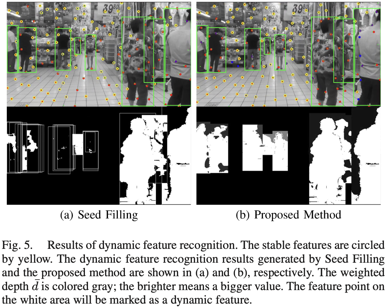
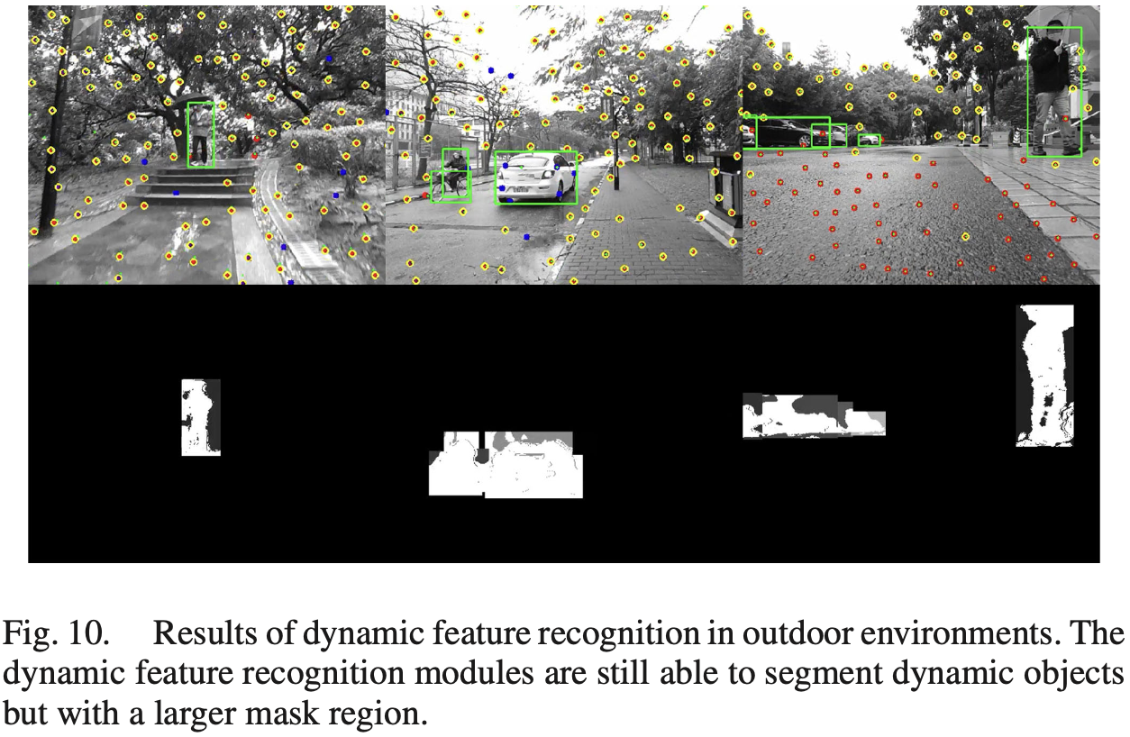
Problem with single-stage object detection: YOLOv3 can be used to detect dynamic elements. But if detected bounding boxes are too large, blindly deleting features in the boxes will result in no available features to provide constraints.
Solution: This paper combines object detection and depth information for feature recognition to achieve performance comparable to semantic measures.
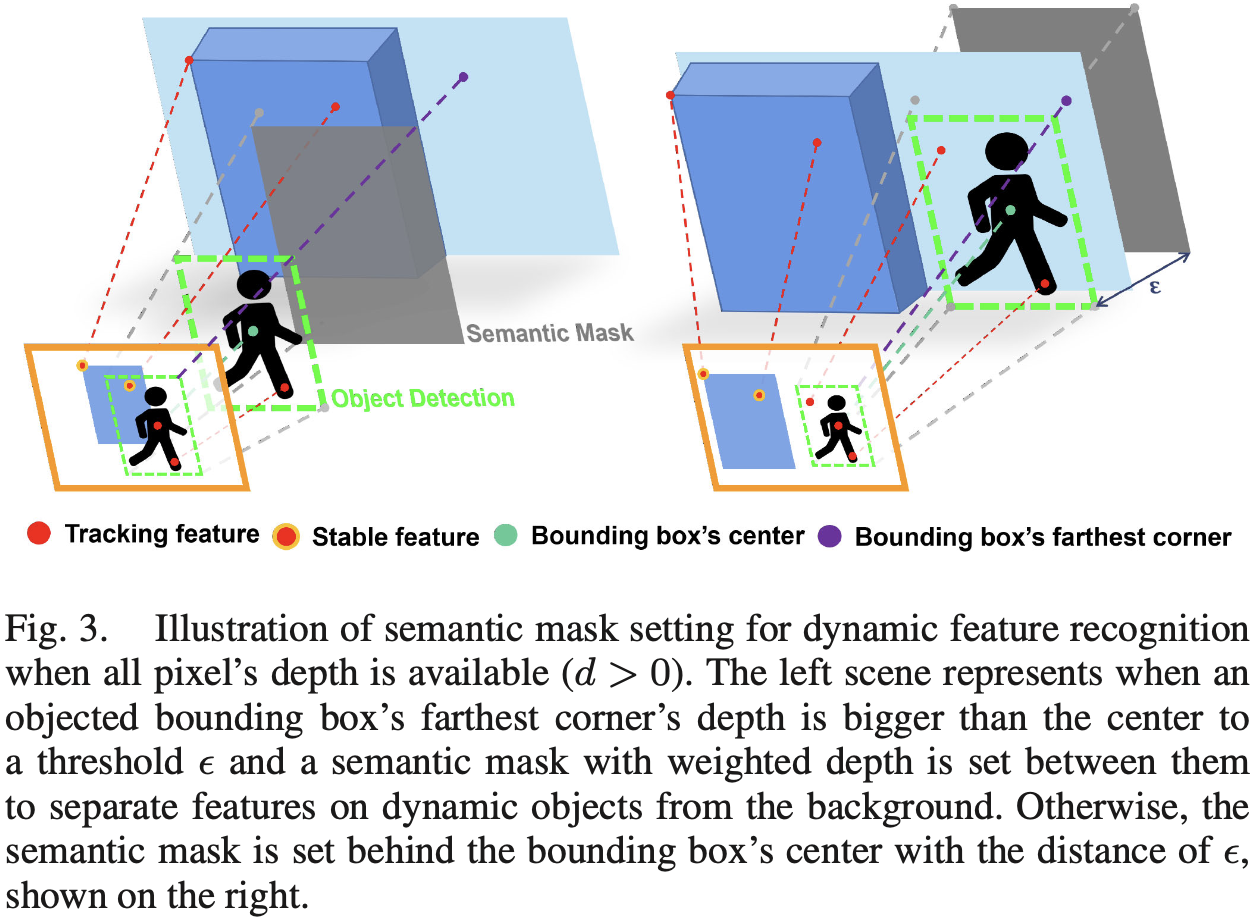
If a pixel’s depth is available, then , otherwise . Considering that the bounding box corners of most dynamic objects correspond to the background points, and the dynamic objects commonly have a relatively large depth gap with the background. The -th dynamic object’s largest background depth is obtained as follow:
are the depth values of the -th object bounding box’s corners. The -th bounding box’s depth threshold is defined as:
is the depth value of the bounding box’s center, is a predefined distance according to the most common dynamic objects’ size in scenes.
On the semantic mask, the area covered by the -th dynamic object bounding box is set to ; the area without dynamic object is set to 0. Each incoming feature’s depth is compared with the corresponding threshold on the semantic mask:
- If , the feature is considered as dynamic;
- Otherwise, the feature is considered as stable.
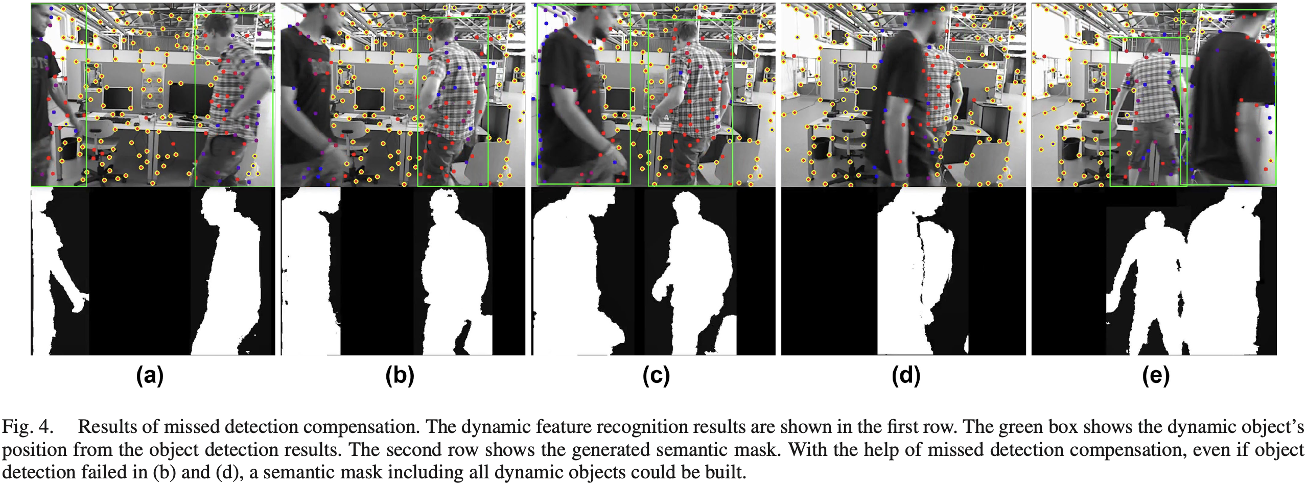
The region where the depth value is smaller than constitutes the generalized semantic mask, as shown in Fig. 4 and Fig. 5(b).
The dynamic features are tracked but not used for pose estimation, different from directly deleting. According to recorded information, each feature from feature tracking thread will be judged whether it is historical dynamic or not.
3.4 Missed Detection Compensation
Since object detection might sometimes fail, Dynamic-VINS uses the previous detection results to predict the following detection result to compensate for missed detections.
Assumption: dynamic objects in adjacent frames have a consistent motion.
Assumed that is the current frame and is previous frame, the pixel velocity of the -th dynamic object between frames is defined as:
is the pixel location of the -th object bounding box’s center in -th frame and -th frame. Weighted predicted velocity is defined as:
If the object fali to be detected in the next frame, the bounding box containing the corners’ pixel locations will be updated based on the predicted velocity as follow:
When the missed detection time is over a threshold, this dynamic object’s compensation will be abandoned, as shown in Fig. 4.
3.5 Moving Consistency Check
Problem: Since object detection can only recognize artificially defined dynamic objects and has a missed detection problem, the state optimization will still be affected by unknown moving objects.
Solution: Dynamic-VINS combines the pose predicted by IMU and the optimized pose in the sliding windows to recognize dynamic features.
Consider the -th feature is first observed in the -th image and observed by other images in sliding window. The average reprojection residual of the feature observation in sliding window is:
is the observation of -th feature in the -th frame; is the 3D location of -th feature in -th frame; and are transforms from camera frame to body frame and from -th body frame to world frame; is the camera projection model. When is over a threshold, the -th feature is considered as dynamic.
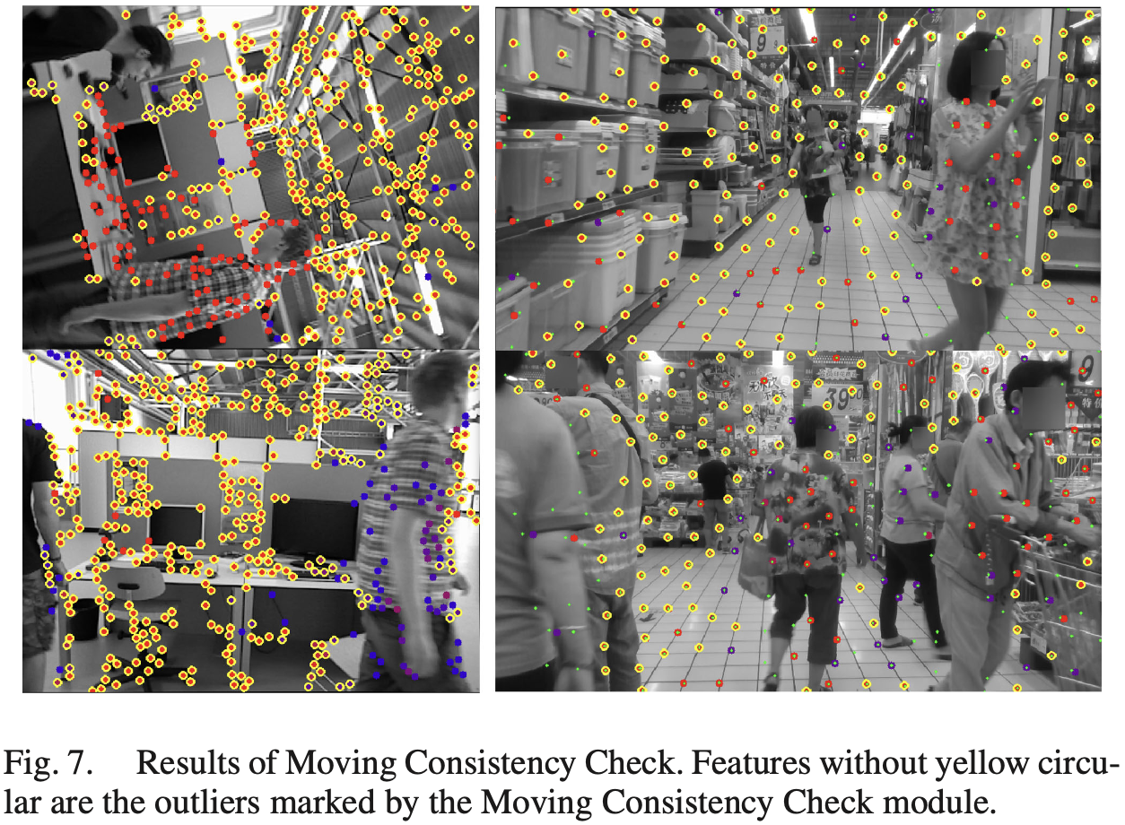
As shown in Fig. 7, module can find out unstable features (red). But some stable feantures are misidentified. A low threshold holds a high recall rate of unstable features.
4 Experimental Results
4.1 Settings
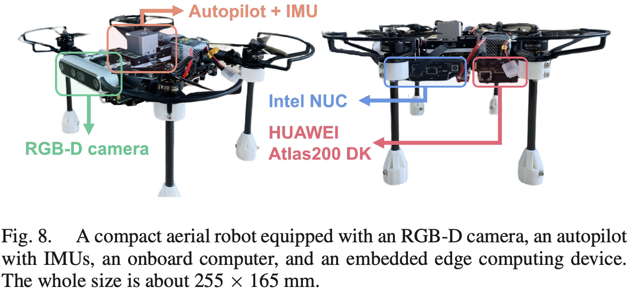
- Datasets: OpenLORIS-Scene, TUM RGB-D
- Baselines: VINS-Mono, VINS-RGBD, ORB-SLAM2, DS-SLAM
- Metrics: RMSE of ATE, T.RPE (Translation of RPE), R.RPE (Rotation of RPE), CR (Correct Rate)
- Platforms: HUAWEI Atlas200 DK, NVIDIA Jetson AGX Xavier
4.2 OpenLORIS-Scene Dataset

4.3 TUM RGB-D Dataset


4.4 Runtime Analysis

4.5 Real-World Experiments
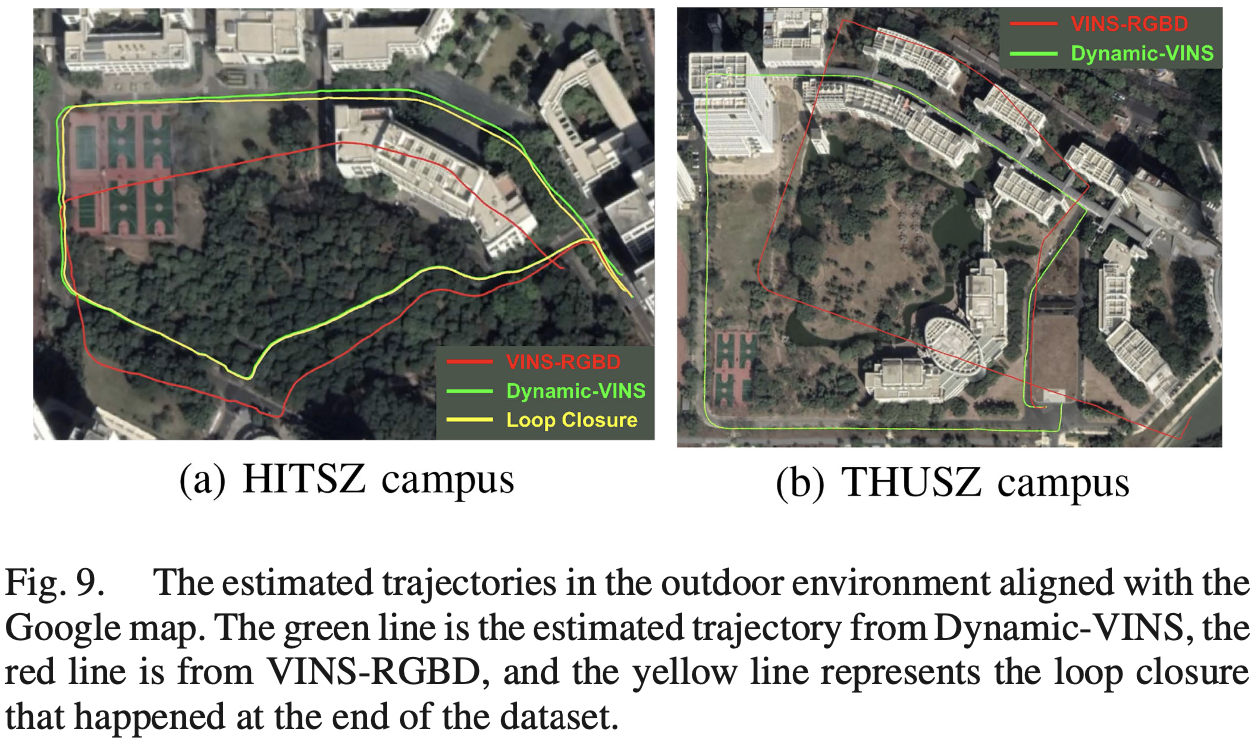
- Ground truth: Google map
5 Appendix
5.1 KLT 光流
- 参考:https://blog.csdn.net/weixin_42905141/article/details/102647830
- 参考:https://leijiezhang001.github.io/KLT/
- 参考:https://www.cnblogs.com/mthoutai/p/7150625.html
基本的光流约束方程(基于灰度不变假设, 和 表示点光流在水平和垂直方向的速度分量):
LK 光流的三个假设:
- 亮度恒定:场景中目标像素在帧间运动时外观上保持不变。
- 时间连续或小运动:图像随时间运动比较缓慢。
- 领域内光流一致:领域内所有像素点的运动是一致的。
KLT 算法本质上也基于上述三个假设,不同于前述直接比较像素点灰度值的作法,KLT 比较像素点周围的窗口像素,来寻找最相似的像素点。
如果推断一个视频的相邻两帧 、 在某局部窗体 上是一样的,则在窗体 内有:。基于 LK 光流的假设 3:
在窗体 上,全部 都往一个方向移动了 ,从而得到 ,即 时刻的 点在 时刻为 。所以寻求匹配的问题可化为对下面的式子寻求最小值:
表达为积分形式:
这个式子的含义即找到两副图像中,在 窗体中,、 的差异。当中 以 为中心, 以 为中心, 为半径的一个矩形窗体间的差异。函数 取最小值,则极值点的导数为 0,即:
由泰勒展开式:
得:
目标式变为:
整理得到:
将式子看为:
为了要使 有解,则 Z 须要满足条件,即 矩阵可逆,在一般情况下,角点具有这样的特点。