关于论文 FAST-LIO2: Fast Direct LiDAR-inertial Odometry (TRO 2022) 的阅读总结。
FAST-LIO2 LiDAR 里程计和建图面临的挑战:
LiDAR 产生的点数量庞大,在计算能力有限的板载平台上实时处理需要高效的算法;
特征(点、线、面)提取容易受到环境影响,且提取效果受到 LiDAR 扫描模式的影响;
LiDAR 连续运动时,点采样会产生运动失真,使用 IMU 解决这一问题又会引入外部偏差;
点云是稀疏且范围较大的,维护稀疏点云地图和进行点云搜索是困难的。
本文提出了两个新技术:增量 K-D 树(incrementa k-d tree)和直接点注册(diret points registration),贡献整理如下:
提出增量 K-D 树数据结构 ikd-Tree,用于高效表示大型稠密点云。除了高效的最近邻查找,ikd-Tree 还支持增量式的地图更新(点插入、删除)和动态的再平衡。
借助 ikd-Tree 计算效率的提高,直接将原始点配准到地图上,实现更准确和可靠的扫描配准。本文将这种基于原始点的配准称为直接法,直接法使系统适用于不同的 LiDAR。
将这两项关键技术集成到 FAST-LIO[1] 中。该系统使用 IMU 通过反向传播补偿每个点的运动,并通过流形迭代卡尔曼滤波器估计系统的完整状态。为了进一步加快计算速度,使用了一个数学等价的卡尔曼增益计算公式,降低计算复杂性,新系统称为 FAST-LIO2。
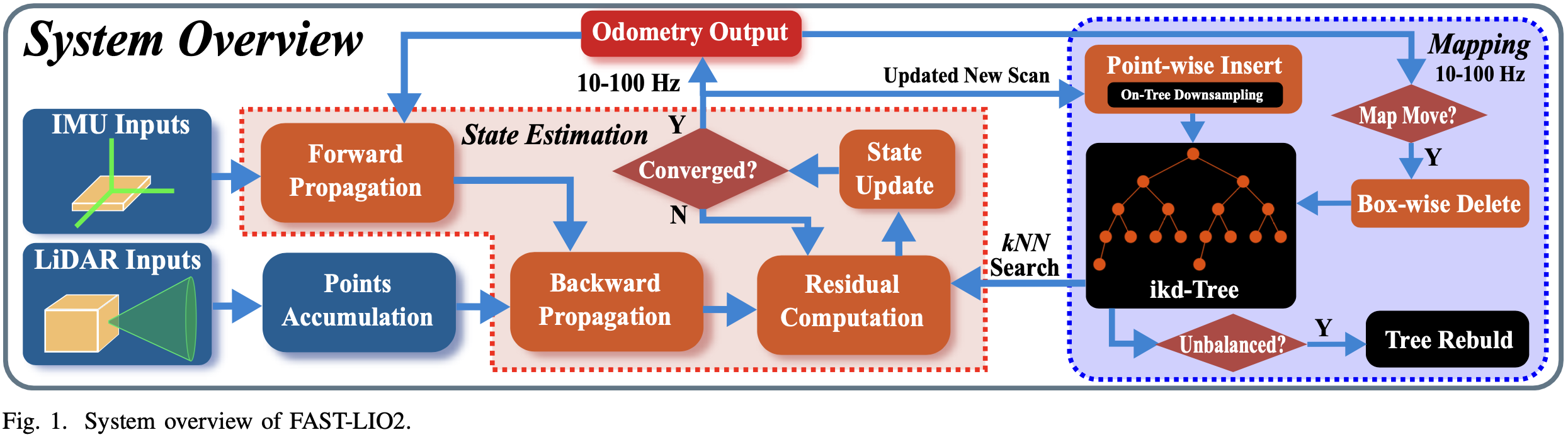
FAST-LIO2 的流程如图-1。
采样的 LiDAR 原始点首先在 10ms 和 100ms 之间的周期内累积,累积的点云称为一次扫描。
新扫描中的点将通过紧耦合迭代卡尔曼滤波框架(红虚线框)注册到大局部地图中保存的地图点。大局部地图中的全局地图点由 ikd-Tree 组织(蓝色虚线框)。
如果当前 LiDAR 的 FoV 范围跨越了地图边界,则将距离 LiDAR 姿态最远的地图区域中的历史点从 ikd-Tree 中删除。因此,ikd-Tree 在一个具有一定长度的大立方体区域(称为 map size)中跟踪所有地图点,并用于状态估计模块中的残差计算。
优化后的姿态最终将新扫描中的点注册到全局框架中,并插入到 ikd-Tree 中,从而合并到地图中。
FAST-LIO2 为继承了 FAST-LIO 的紧耦合迭代卡尔曼滤波器。
取第一个 IMU 帧(IMU 帧记为 I I I G G G I T L = ( I R L , I p L ) {}^I \mathbf{T}_L = ({}^I \mathbf{R}_L, {}^I \mathbf{p}_L) I T L = ( I R L , I p L )
G R ˙ I = G R I ⌊ ω m − b ω − n ω ⌋ ∧ , G p ˙ I = G v I , G v ˙ I = G R I ( a m − b a − n a ) + G g b ˙ ω = n b ω , b ˙ a = n b a , G g ˙ = 0 , I R ˙ L = 0 , I p ˙ L = 0 (1) \begin{aligned}
{ }^G \dot{\mathbf{R}}_I & ={ }^G \mathbf{R}_I\left\lfloor\boldsymbol{\omega}_m-\mathbf{b}_{\boldsymbol{\omega}}-\mathbf{n}_{\boldsymbol{\omega}}\right\rfloor_{\wedge},{ }^G \dot{\mathbf{p}}_I={ }^G \mathbf{v}_I, \\
{ }^G \dot{\mathbf{v}}_I & ={ }^G \mathbf{R}_I\left(\mathbf{a}_m-\mathbf{b}_{\mathbf{a}}-\mathbf{n}_{\mathbf{a}}\right)+{ }^G \mathbf{g} \\
\dot{\mathbf{b}}_{\boldsymbol{\omega}} & =\mathbf{n}_{\mathbf{b} \boldsymbol{\omega}}, \dot{\mathbf{b}}_{\mathbf{a}}=\mathbf{n}_{\mathbf{b a}}, \\
{ }^G \dot{\mathbf{g}} & =\mathbf{0},{ }^I \dot{\mathbf{R}}_L=\mathbf{0},{ }^I \dot{\mathbf{p}}_L=\mathbf{0}
\end{aligned}
\tag{1}
G R ˙ I G v ˙ I b ˙ ω G g ˙ = G R I ⌊ ω m − b ω − n ω ⌋ ∧ , G p ˙ I = G v I , = G R I ( a m − b a − n a ) + G g = n b ω , b ˙ a = n b a , = 0 , I R ˙ L = 0 , I p ˙ L = 0 ( 1 )
G R I , G p I { }^G \mathbf{R}_I, { }^G \mathbf{p}_I G R I , G p I G g { }^G \mathbf{g} G g a m , ω m \mathbf{a}_m, \boldsymbol{\omega}_m a m , ω m ⌊ a ⌋ ∧ \lfloor \mathbf{a} \rfloor_{\wedge} ⌊ a ⌋ ∧ a ∈ R 3 \mathbf{a} \in \mathbb{R}^3 a ∈ R 3
记 i i i Δ t \Delta t Δ t ⊞ / ⊟ \boxplus / \boxminus ⊞ / ⊟
x i + 1 = x i ⊞ ( Δ t f ( x i , u i , w i ) ) (2) \mathbf{x}_{i+1} = \mathbf{x}_i \boxplus (\Delta t \mathbf{f}(\mathbf{x}_i, \mathbf{u}_i, \mathbf{w}_i)) \\
\tag{2}
x i + 1 = x i ⊞ ( Δ t f ( x i , u i , w i ) ) ( 2 )
函数 f \mathbf{f} f x \mathbf{x} x u \mathbf{u} u w \mathbf{w} w
M ≜ S O ( 3 ) × R 15 × S O ( 3 ) × R 3 ; dim ( M ) = 24 x ≜ [ G R I T G p I T G v I T b ω T b a T G g T I R L T I p L T ] T ∈ M u ≜ [ ω m T a m T ] T , w ≜ [ n ω T n a T n b ω T n b a T ] T f ( x , u , w ) = [ ω m − b ω − n ω G v I + 1 2 ( G R I ( a m − b a − n a ) + G g ) Δ t R I ( a m − b a − n a ) + G g n b ω n b a 0 3 × 1 0 3 × 1 0 3 × 1 ] ∈ R 24 (3) \begin{aligned}
& \mathcal{M} \triangleq S O(3) \times \mathbb{R}^{15} \times S O(3) \times \mathbb{R}^3 ; \operatorname{dim}(\mathcal{M})=24 \\
& \mathbf{x} \triangleq\left[\begin{array}{llllllll}
{ }^G \mathbf{R}_I^T & { }^G \mathbf{p}_I^T & { }^G \mathbf{v}_I^T & \mathbf{b}_{\boldsymbol{\omega}}^T & \mathbf{b}_{\mathbf{a}}^T & { }^G \mathbf{g}^T & { }^I \mathbf{R}_L^T & { }^I \mathbf{p}_L^T
\end{array}\right]^T \in \mathcal{M} \\
& \mathbf{u} \triangleq\left[\begin{array}{ll}
\boldsymbol{\omega}_m^T & \mathbf{a}_m^T
\end{array}\right]^T, \mathbf{w} \triangleq\left[\begin{array}{llll}
\mathbf{n}_{\boldsymbol{\omega}}^T & \mathbf{n}_{\mathbf{a}}^T & \mathbf{n}_{\mathbf{b} \boldsymbol{\omega}}^T & \mathbf{n}_{\mathbf{b a}}^T
\end{array}\right]^T \\
& \mathbf{f}(\mathbf{x}, \mathbf{u}, \mathbf{w})=\left[\begin{array}{c}
\boldsymbol{\omega}_m-\mathbf{b}_{\boldsymbol{\omega}}-\mathbf{n}_{\boldsymbol{\omega}} \\
{ }^G \mathbf{v}_I+\frac{1}{2}\left({ }^G \mathbf{R}_I\left(\mathbf{a}_m-\mathbf{b}_{\mathbf{a}}-\mathbf{n}_{\mathbf{a}}\right)+{ }^G \mathbf{g}\right) \Delta t \\
\mathbf{R}_I\left(\mathbf{a}_m-\mathbf{b}_{\mathbf{a}}-\mathbf{n}_{\mathbf{a}}\right)+{ }^G \mathbf{g} \\
\mathbf{n}_{\mathbf{b} \boldsymbol{\omega}} \\
\mathbf{n}_{\mathbf{b a}} \\
\mathbf{0}_{3 \times 1} \\
\mathbf{0}_{3 \times 1} \\
\mathbf{0}_{3 \times 1}
\end{array}\right] \in \mathbb{R}^{24} \\
&
\end{aligned}
\tag{3}
M ≜ S O ( 3 ) × R 1 5 × S O ( 3 ) × R 3 ; d i m ( M ) = 2 4 x ≜ [ G R I T G p I T G v I T b ω T b a T G g T I R L T I p L T ] T ∈ M u ≜ [ ω m T a m T ] T , w ≜ [ n ω T n a T n b ω T n b a T ] T f ( x , u , w ) = ⎣ ⎢ ⎢ ⎢ ⎢ ⎢ ⎢ ⎢ ⎢ ⎢ ⎢ ⎡ ω m − b ω − n ω G v I + 2 1 ( G R I ( a m − b a − n a ) + G g ) Δ t R I ( a m − b a − n a ) + G g n b ω n b a 0 3 × 1 0 3 × 1 0 3 × 1 ⎦ ⎥ ⎥ ⎥ ⎥ ⎥ ⎥ ⎥ ⎥ ⎥ ⎥ ⎤ ∈ R 2 4 ( 3 )
LiDAR 通常逐个进行点采样。因此,LiDAR 连续运动时会以不同的姿态对点进行采样。为了纠正这种扫描内运动,采用 [1] 中提出的反向传播,根据 IMU 测量值估计扫描中每个点的 LiDAR 姿态相对于扫描结束时间的姿态。估计的相对姿态使得能够基于扫描中每个单独点的精确采样时间,将所有点投影到扫描结束时间。因此,可以得到扫描中的点在扫描结束时被同时采样。
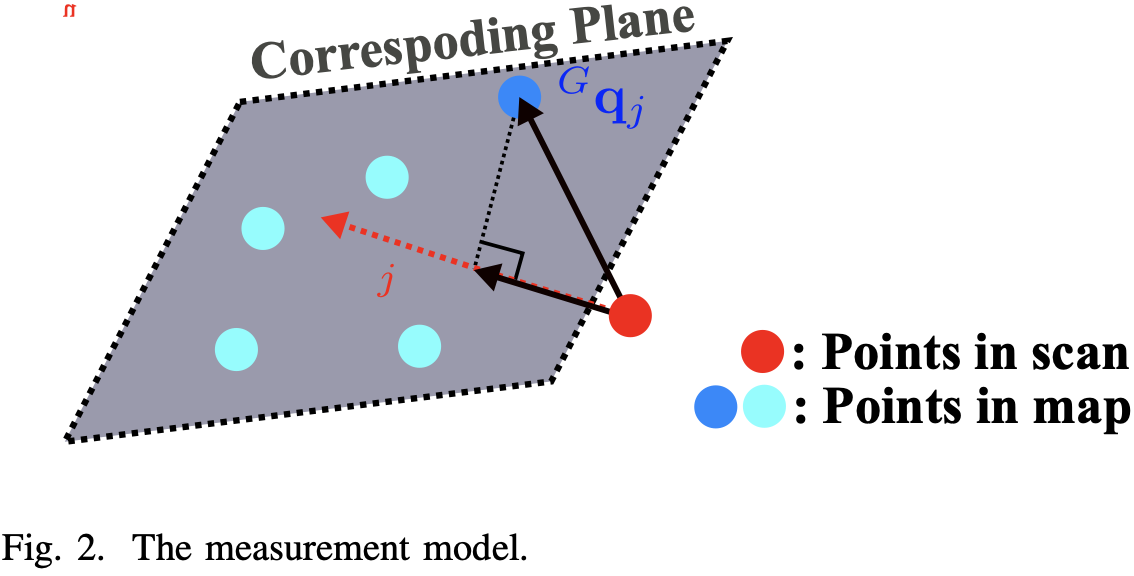
记 k k k L L L k k k { L p j , j = 1 , . . . , m } \lbrace {}^L \mathbf{p}_j, j = 1, ..., m \rbrace { L p j , j = 1 , . . . , m } L p j {}^L \mathbf{p}_j L p j L n j {}^L \mathbf{n}_j L n j
L p j g t = L p j + L n j (3) {}^L \mathbf{p}_j^{gt} = {}^L \mathbf{p}_j + {}^L \mathbf{n}_j
\tag{3}
L p j g t = L p j + L n j ( 3 )
如图-2,真实的点通过位姿应该准确地落在地图的一个局部小平面段上:
0 = G u j T ( G T I k I T L ( L p j + L n j ) − G q j ) (4) \mathbf{0} = {}^G \mathbf{u}_j^T ({}^G \mathbf{T}_{I_k} {}^I \mathbf{T}_L ({}^L \mathbf{p}_j + {}^L \mathbf{n}_j) - {}^G \mathbf{q}_j)
\tag{4}
0 = G u j T ( G T I k I T L ( L p j + L n j ) − G q j ) ( 4 )
G u j {}^G \mathbf{u}_j G u j G q j T {}^G \mathbf{q}_j^T G q j T G T I k , I T L {}^G \mathbf{T}_{I_k}, {}^I \mathbf{T}_L G T I k , I T L x k \mathbf{x}_k x k j j j
0 = h j ( x k , L p j + L n j ) (5) \mathbf{0} = \mathbf{h}_j(\mathbf{x}_k, {}^L \mathbf{p}_j + {}^L \mathbf{n}_j)
\tag{5}
0 = h j ( x k , L p j + L n j ) ( 5 )
(5) 定义了状态 x k \mathbf{x}_k x k
基于流形 M ≜ S O ( 3 ) × R 15 × S O ( 3 ) × R 3 \mathcal{M} \triangleq SO(3) \times \mathbb{R}^{15} \times SO(3) \times \mathbb{R}^3 M ≜ S O ( 3 ) × R 1 5 × S O ( 3 ) × R 3 M \mathcal{M} M
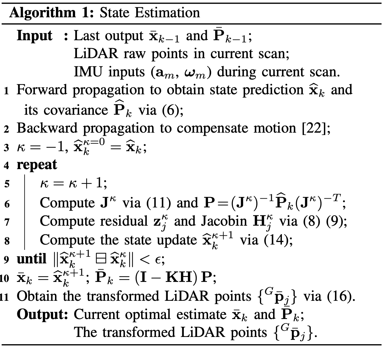
设前一个扫描的优化后状态估计为 x ˉ k − 1 \bar{\mathbf{x}}_{k-1} x ˉ k − 1 P ˉ k − 1 \bar{\mathbf{P}}_{k-1} P ˉ k − 1 w i \mathbf{w}_i w i
x ^ i + 1 = x ^ i ⊞ ( Δ t f ( x ^ i , u i , 0 ) ) ; x ^ 0 = x ˉ k − 1 P ^ i + 1 = F x ~ i P ^ i F x ~ i T + F w i Q i F w i T ; P ^ 0 = P ˉ k − 1 (6) \begin{aligned}
&\widehat{\mathbf{x}}_{i+1} = \widehat{\mathbf{x}}_i \boxplus (\Delta t \mathbf{f}(\widehat{\mathbf{x}}_i, \mathbf{u}_i, \mathbf{0})); \widehat{\mathbf{x}}_0 = \bar{\mathbf{x}}_{k-1} \\
&\widehat{\mathbf{P}}_{i+1} = \mathbf{F}_{\widetilde{\mathbf{x}}_{i}} \widehat{\mathbf{P}}_i \mathbf{F}_{\widetilde{\mathbf{x}}_{i}}^T + \mathbf{F}_{\mathbf{w}_i} \mathbf{Q}_i \mathbf{F}_{\mathbf{w}_i}^T; \widehat{\mathbf{P}}_0 = \bar{\mathbf{P}}_{k-1}
\end{aligned}
\tag{6}
x i + 1 = x i ⊞ ( Δ t f ( x i , u i , 0 ) ) ; x 0 = x ˉ k − 1 P i + 1 = F x i P i F x i T + F w i Q i F w i T ; P 0 = P ˉ k − 1 ( 6 )
其中 Q i \mathbf{Q}_i Q i w i \mathbf{w}_i w i F x ~ i \mathbf{F}_{\widetilde{\mathbf{x}}_{i}} F x i F w i \mathbf{F}_{\mathbf{w}_i} F w i
F x ~ i = ∂ ( x i + 1 ⊟ x ^ i + 1 ) ∂ x ~ i ∣ x ~ i = 0 , w i = 0 F w i = ∂ ( x i + 1 ⊟ x ^ i + 1 ) ∂ w i ∣ x ~ i = 0 , w i = 0 (7) \begin{aligned}
&\mathbf{F}_{\widetilde{\mathbf{x}}_{i}} = \left. \frac{\partial (\mathbf{x}_{i+1} \boxminus \widehat{\mathbf{x}}_{i+1})}{\partial \widetilde{\mathbf{x}}_i} \right|_{\widetilde{\mathbf{x}}_i = \mathbf{0}, \mathbf{w}_i = \mathbf{0}} \\
&\mathbf{F}_{\mathbf{w}_i} = \left. \frac{\partial (\mathbf{x}_{i+1} \boxminus \widehat{\mathbf{x}}_{i+1})}{\partial \mathbf{w}_i} \right|_{\widetilde{\mathbf{x}}_i = \mathbf{0}, \mathbf{w}_i = \mathbf{0}}
\end{aligned}
\tag{7}
F x i = ∂ x i ∂ ( x i + 1 ⊟ x i + 1 ) ∣ ∣ ∣ ∣ x i = 0 , w i = 0 F w i = ∂ w i ∂ ( x i + 1 ⊟ x i + 1 ) ∣ ∣ ∣ ∣ x i = 0 , w i = 0 ( 7 )
前向传播持续到新扫描(第 k k k x ^ k , P ^ k \widehat{\mathbf{x}}_k, \widehat{\mathbf{P}}_k x k , P k
设当前迭代的状态估计为 x ^ k κ \widehat{\mathbf{x}}_k^{\kappa} x k κ κ = 0 \kappa = 0 κ = 0 x ^ k κ = x ^ k \widehat{\mathbf{x}}_k^{\kappa} = \widehat{\mathbf{x}}_k x k κ = x k L p j {}^L \mathbf{p}_j L p j G p ^ j = G T ^ I k κ I T ^ L k κ L p j {}^G \widehat{\mathbf{p}}_j = {}^G \widehat{\mathbf{T}}_{I_k}^{\kappa} {}^I \widehat{\mathbf{T}}_{L_k}^{\kappa} {}^L \mathbf{p}_j G p j = G T I k κ I T L k κ L p j G u j {}^G \mathbf{u}_j G u j G q j {}^G \mathbf{q}_j G q j
测量方程 (5) 在 x ^ k κ \widehat{\mathbf{x}}_k^{\kappa} x k κ
0 = h j ( x k , L n j ) ≃ h j ( x ^ k κ , 0 ) + H j κ x ~ k κ + v j = z j κ + H j κ x ~ k κ + v j (8) \begin{aligned}
\mathbf{0} & =\mathbf{h}_j\left(\mathbf{x}_k,{ }^L \mathbf{n}_j\right) \simeq \mathbf{h}_j\left(\widehat{\mathbf{x}}_k^\kappa, \mathbf{0}\right)+\mathbf{H}_j^\kappa \widetilde{\mathbf{x}}_k^\kappa+\mathbf{v}_j \\
& =\mathbf{z}_j^\kappa+\mathbf{H}_j^\kappa \widetilde{\mathbf{x}}_k^\kappa+\mathbf{v}_j
\end{aligned}
\tag{8}
0 = h j ( x k , L n j ) ≃ h j ( x k κ , 0 ) + H j κ x k κ + v j = z j κ + H j κ x k κ + v j ( 8 )
其中 x ~ k κ = x k ⊟ x ^ k κ \widetilde{\mathbf{x}}_k^{\kappa} = \mathbf{x}_k \boxminus \widehat{\mathbf{x}}_k^{\kappa} x k κ = x k ⊟ x k κ H j κ \mathbf{H}_j^{\kappa} H j κ 0 = h j ( x ^ k κ ⊞ x ~ k κ , L n j ) \mathbf{0} =\mathbf{h}_j\left(\widehat{\mathbf{x}}_k^{\kappa} \boxplus \widetilde{\mathbf{x}}_k^{\kappa},{ }^L \mathbf{n}_j\right) 0 = h j ( x k κ ⊞ x k κ , L n j ) x ~ k κ \widetilde{\mathbf{x}}_k^{\kappa} x k κ v j ∈ N ( 0 , R j ) \mathbf{v}_j \in \mathcal{N}(\mathbf{0}, \mathbf{R}_j) v j ∈ N ( 0 , R j ) z j κ \mathbf{z}_j^{\kappa} z j κ
z j κ = h j ( x ^ k κ , 0 ) = G u j T ( G T ^ I k κ I T ^ L k κ L p j − G q j ) (9) \mathbf{z}_j^{\kappa} = \mathbf{h}_j(\widehat{\mathbf{x}}_k^{\kappa}, \mathbf{0}) = {}^G \mathbf{u}_j^T ({}^G \widehat{\mathbf{T}}_{I_k}^{\kappa} {}^I \widehat{\mathbf{T}}_{L_k}^{\kappa} {}^L \mathbf{p}_j - {}^G \mathbf{q}_j)
\tag{9}
z j κ = h j ( x k κ , 0 ) = G u j T ( G T I k κ I T L k κ L p j − G q j ) ( 9 )
x ^ k , P ^ k \widehat{\mathbf{x}}_k, \widehat{\mathbf{P}}_k x k , P k
x k ⊟ x ^ k = ( x ^ k κ ⊞ x ~ k κ ) ⊟ x ^ k = x ^ k κ ⊟ x ^ k + J κ x ~ k κ ∼ N ( 0 , P ^ k ) (10) \mathbf{x}_k \boxminus \widehat{\mathbf{x}}_k = (\widehat{\mathbf{x}}_k^{\kappa} \boxplus \widetilde{\mathbf{x}}_k^{\kappa}) \boxminus \widehat{\mathbf{x}}_k = \widehat{\mathbf{x}}_k^{\kappa} \boxminus \widehat{\mathbf{x}}_k + \mathbf{J}^{\kappa} \widetilde{\mathbf{x}}_k^{\kappa} \sim \mathcal{N}(\mathbf{0}, \widehat{\mathbf{P}}_k)
\tag{10}
x k ⊟ x k = ( x k κ ⊞ x k κ ) ⊟ x k = x k κ ⊟ x k + J κ x k κ ∼ N ( 0 , P k ) ( 1 0 )
J κ \mathbf{J}^{\kappa} J κ ( x ^ k κ ⊞ x ~ k κ ) ⊟ x ^ k (\widehat{\mathbf{x}}_k^{\kappa} \boxplus \widetilde{\mathbf{x}}_k^{\kappa}) \boxminus \widehat{\mathbf{x}}_k ( x k κ ⊞ x k κ ) ⊟ x k x ~ k κ \widetilde{\mathbf{x}}_k^{\kappa} x k κ
J κ = [ A ( δ G θ I k ) − T 0 3 × 15 0 3 × 3 0 3 × 3 0 15 × 3 I 15 × 15 0 3 × 3 0 3 × 3 0 3 × 3 0 3 × 15 A ( δ I θ L k ) − T 0 3 × 3 0 3 × 3 0 3 × 15 0 3 × 3 I 3 × 3 ] (11) \mathbf{J}^\kappa=\left[\begin{array}{cccc}
\mathbf{A}\left(\delta^G \boldsymbol{\theta}_{I_k}\right)^{-T} & \mathbf{0}_{3 \times 15} & \mathbf{0}_{3 \times 3} & \mathbf{0}_{3 \times 3} \\
\mathbf{0}_{15 \times 3} & \mathbf{I}_{15 \times 15} & \mathbf{0}_{3 \times 3} & \mathbf{0}_{3 \times 3} \\
\mathbf{0}_{3 \times 3} & \mathbf{0}_{3 \times 15} & \mathbf{A}\left(\delta^I \boldsymbol{\theta}_{L_k}\right)^{-T} & \mathbf{0}_{3 \times 3} \\
\mathbf{0}_{3 \times 3} & \mathbf{0}_{3 \times 15} & \mathbf{0}_{3 \times 3} & \mathbf{I}_{3 \times 3}
\end{array}\right]
\tag{11}
J κ = ⎣ ⎢ ⎢ ⎡ A ( δ G θ I k ) − T 0 1 5 × 3 0 3 × 3 0 3 × 3 0 3 × 1 5 I 1 5 × 1 5 0 3 × 1 5 0 3 × 1 5 0 3 × 3 0 3 × 3 A ( δ I θ L k ) − T 0 3 × 3 0 3 × 3 0 3 × 3 0 3 × 3 I 3 × 3 ⎦ ⎥ ⎥ ⎤ ( 1 1 )
A ( ⋅ ) − 1 \mathbf{A}(\cdot)^{-1} A ( ⋅ ) − 1 δ G θ I k = G R ^ I k κ ⊟ G R ^ I k \delta {}^G \boldsymbol{\theta}_{I_k} = {}^G \widehat{\mathbf{R}}_{I_k}^{\kappa} \boxminus {}^G \widehat{\mathbf{R}}_{I_k} δ G θ I k = G R I k κ ⊟ G R I k δ I θ L k = I R ^ L k κ ⊟ I R ^ L k \delta {}^I \boldsymbol{\theta}_{L_k} = {}^I \widehat{\mathbf{R}}_{L_k}^{\kappa} \boxminus {}^I \widehat{\mathbf{R}}_{L_k} δ I θ L k = I R L k κ ⊟ I R L k x ^ k κ = x ^ k , J κ = I \widehat{\mathbf{x}}_k^{\kappa} = \widehat{\mathbf{x}}_k, \mathbf{J}^{\kappa} = \mathbf{I} x k κ = x k , J κ = I
对于先验分布,根据测量 (8) 可以得到状态分布:
− v j = z j κ + H j κ x ~ k κ ∼ N ( 0 , R j ) (12) - \mathbf{v}_j = \mathbf{z}_j^\kappa + \mathbf{H}_j^\kappa \widetilde{\mathbf{x}}_k^\kappa \sim \mathcal{N}(\mathbf{0}, \mathbf{R}_j)
\tag{12}
− v j = z j κ + H j κ x k κ ∼ N ( 0 , R j ) ( 1 2 )
联合 (10) 和 (12) 得到状态 x k \mathbf{x}_k x k x ~ k \widetilde{\mathbf{x}}_k x k
min x ~ k κ ( ∥ x k ⊟ x ^ k ∥ P ^ k 2 + ∑ j = 1 m ∥ z j κ + H j κ x ~ k κ ∥ R j 2 ) (13) \min_{\widetilde{\mathbf{x}}_k^{\kappa}} \left( \| \mathbf{x}_k \boxminus \widehat{\mathbf{x}}_k \|^2_{\widehat{\mathbf{P}}_k} + \sum_{j=1}^m \| \mathbf{z}_j^{\kappa} + \mathbf{H}_j^{\kappa} \widetilde{\mathbf{x}}_k^{\kappa} \|^2_{\mathbf{R}_j} \right)
\tag{13}
x k κ min ( ∥ x k ⊟ x k ∥ P k 2 + j = 1 ∑ m ∥ z j κ + H j κ x k κ ∥ R j 2 ) ( 1 3 )
MAP 问题可以通过卡尔曼滤波解决(取 H = [ H 1 κ , … , H m κ ] T \mathbf{H} = [\mathbf{H}_1^{\kappa}, \dots, \mathbf{H}_m^{\kappa}]^T H = [ H 1 κ , … , H m κ ] T R = diag ( R 1 , … , R m ) \mathbf{R} = \operatorname{diag}(\mathbf{R}_1, \dots, \mathbf{R}_m) R = d i a g ( R 1 , … , R m ) P = ( J κ ) − 1 P ^ k ( J κ ) − T \mathbf{P} = (\mathbf{J^{\kappa}})^{-1} \widehat{\mathbf{P}}_k (\mathbf{J}^{\kappa})^{-T} P = ( J κ ) − 1 P k ( J κ ) − T z k κ = [ z 1 κ T , … , z m κ T ] T \mathbf{z}_k^{\kappa} = [{\mathbf{z}_1^{\kappa}}^T, \dots, {\mathbf{z}_m^{\kappa}}^T]^T z k κ = [ z 1 κ T , … , z m κ T ] T
K = ( H T R − 1 H + P − 1 ) − 1 H T R − 1 x ^ k κ + 1 = x ^ k κ ⊞ ( − K z k κ − ( I − K H ) ( J κ ) − 1 ( x ^ k κ ⊟ x ^ k ) ) (14) \begin{aligned}
&\mathbf{K} = (\mathbf{H}^T \mathbf{R}^{-1} \mathbf{H} + \mathbf{P}^{-1})^{-1} \mathbf{H}^T \mathbf{R}^{-1} \\
&\widehat{\mathbf{x}}_k^{\kappa+1} = \widehat{\mathbf{x}}_k^{\kappa} \boxplus \left(- \mathbf{K} \mathbf{z}_k^{\kappa} - (\mathbf{I} - \mathbf{KH})(\mathbf{J}^{\kappa})^{-1}(\widehat{\mathbf{x}}_k^{\kappa} \boxminus \widehat{\mathbf{x}}_k) \right)
\end{aligned}
\tag{14}
K = ( H T R − 1 H + P − 1 ) − 1 H T R − 1 x k κ + 1 = x k κ ⊞ ( − K z k κ − ( I − K H ) ( J κ ) − 1 ( x k κ ⊟ x k ) ) ( 1 4 )
迭代上述过程至收敛后,优化的状态和协方差为:
x ^ k = x ^ k κ + 1 , P ^ k = ( I − K H ) P (15) \widehat{\mathbf{x}}_k = \widehat{\mathbf{x}}_k^{\kappa+1}, \widehat{\mathbf{P}}_k = (\mathbf{I} - \mathbf{KH}) \mathbf{P}
\tag{15}
x k = x k κ + 1 , P k = ( I − K H ) P ( 1 5 )
透过优化状态,可以将第 k k k L p j {}^L \mathbf{p}_j L p j
G p ˉ j = G T ˉ I k I T ˉ L k L p j ; j = 1 , . . . , m (16) {}^G \bar{\mathbf{p}}_j = {}^G \bar{\mathbf{T}}_{I_k} {}^I \bar{\mathbf{T}}_{L_k} {}^L \mathbf{p}_j; \quad j = 1, ..., m
\tag{16}
G p ˉ j = G T ˉ I k I T ˉ L k L p j ; j = 1 , . . . , m ( 1 6 )
转换后的点集 { G p ˉ j } \lbrace {}^G \bar{\mathbf{p}}_j \rbrace { G p ˉ j }
整个状态估计算法如下:
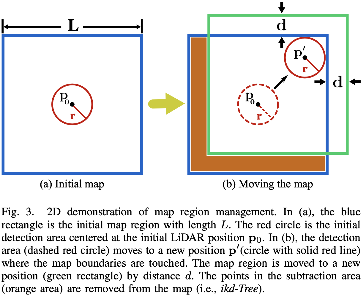
地图点被组织成 ikd-Tree,通过合并新的点云扫描来动态增长。为防止地图尺寸失控,ikd-Tree 只保留 LiDAR 当前位置周围一个长度 L L L
将地图区域初始化为长度 L L L p 0 \mathbf{p}_0 p 0 r = γ R r = \gamma R r = γ R R R R γ \gamma γ
当 LiDAR 移动到新位置 p ′ \mathbf{p}^{\prime} p ′ d = ( γ − 1 ) R d = (\gamma−1)R d = ( γ − 1 ) R
对于新的地图区域和旧的地图区域之间的差值区域,所有的点都将通过 4.3 中的算法-3 从 ikd-Tree 中删除。
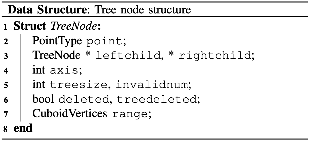
ikd-Tree 为二叉搜索树,数据结构如下:
由于点对应于 ikd-Tree 中的单个节点:
点的信息(如点坐标、强度)存储在 point 中。leftchild和 rightchild 是指向左右子节点的指针。
用于分割空间的分割轴存储在 axis 中。
根在当前节点的(子)树的节点数(包括有效节点和无效节点)保存在 treesize 中。
当从地图中删除点时,这些节点不会立即从树中删除,只将 deleted 设为 true。
如果根在当前节点的整个(子)树被删除,则 treedeleted 设为 true。
从(子)树中删除的点数为 invalidnum。
range 存储(子)树上点的范围信息,解释为一个包含所有点的轴向外接长方体。
ikd-Tree 的构建过程与构建 KD 树类似。ikd-Tree 沿着最长维度递归地在中点对空间进行分割,直到子空间中只剩下一个点。在构造过程中对数据结构中的属性进行初始化,包括计算树的大小和(子)树的范围信息。
ikd-Tree 支持两种增量操作:逐点操作和逐框(box-wise)操作:
逐点操作在 KD 树之间插入、删除或重新插入单个点;
逐框操作在给定的轴对齐长方体中插入、删除或重新插入所有点。
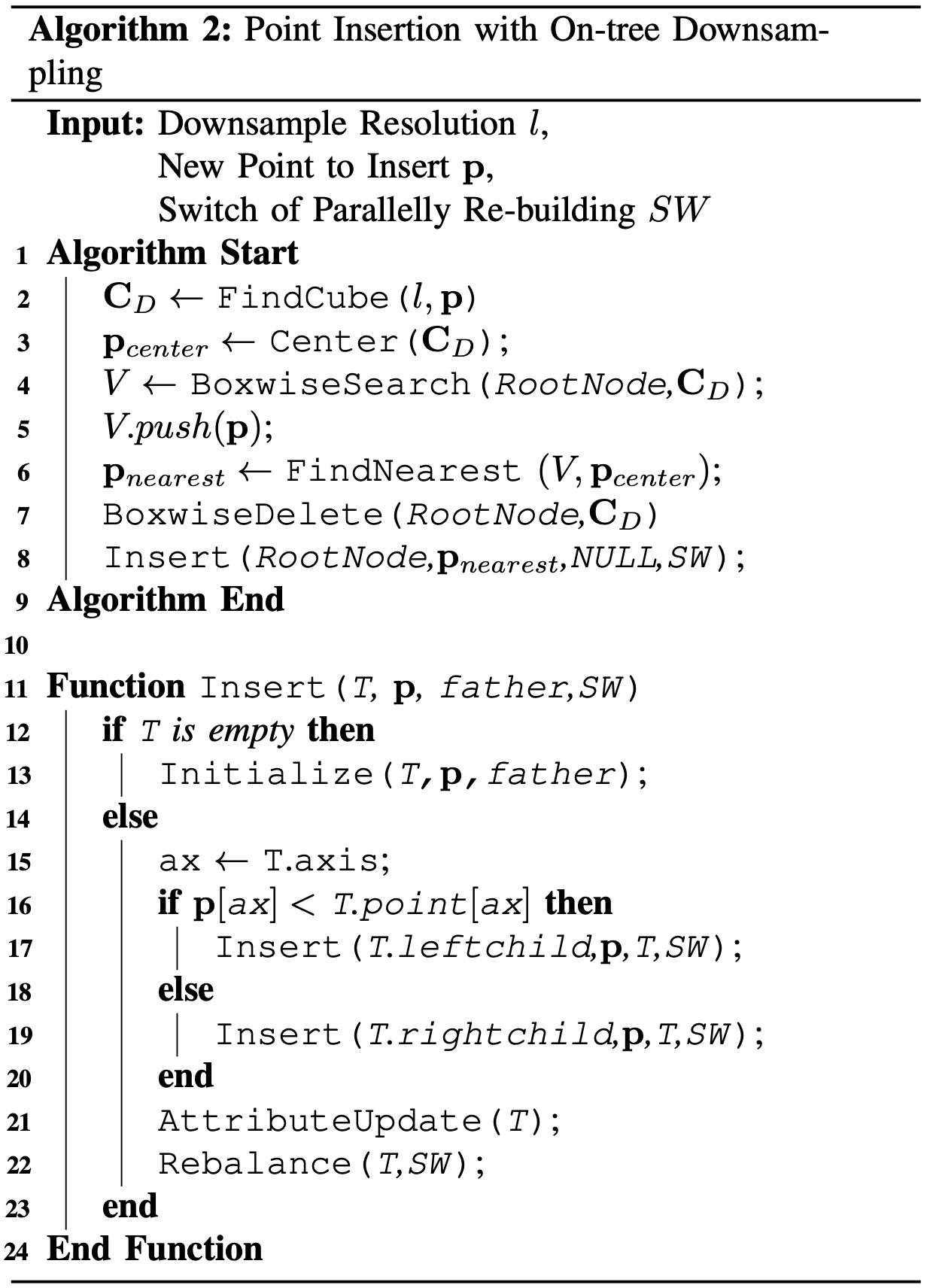
ikd-Tree 支持点插入和地图下采样,具体算法见算法-2。
对于从算法-1 得到的点 p ∈ { G p ˉ j } \mathbf{p} \in \lbrace{}^G \bar{\mathbf{p}}_j \rbrace p ∈ { G p ˉ j } l l l l l l p \mathbf{p} p C D \mathbf{C}_D C D C D \mathbf{C}_D C D p c e n t e r \mathbf{p}_{center} p c e n t e r C D \mathbf{C}_D C D V V V V V V p \mathbf{p} p V V V p c e n t e r \mathbf{p}_{center} p c e n t e r C D \mathbf{C}_D C D p n e a r e s t \mathbf{p}_{nearest} p n e a r e s t BoxwiseSearch 类似于算法-3 的 BoxwiseDelete。
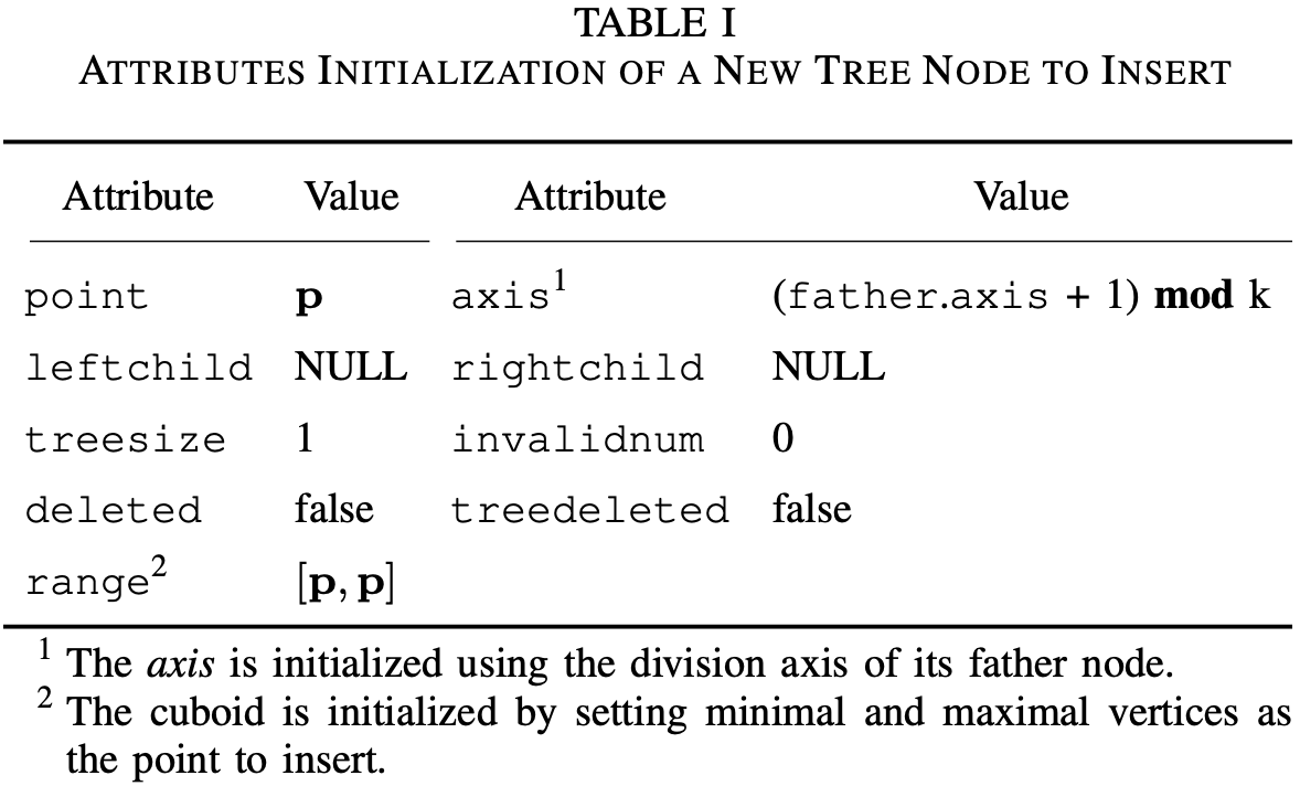
ikd-Tree 上的点插入(第 11-24 行)递归实现,算法从根节点开始向下搜索,直到找到一个空节点来添加新节点(第 12-14 行)。新叶节点的初始化如表-1:
访问过的节点的属性(如 treesize,range)会被更新(第 21 行)。对于更新后的子树,检查并维护平衡(第 22 行),以保持 ikd-Tree 的平衡性(参见 4.4)。
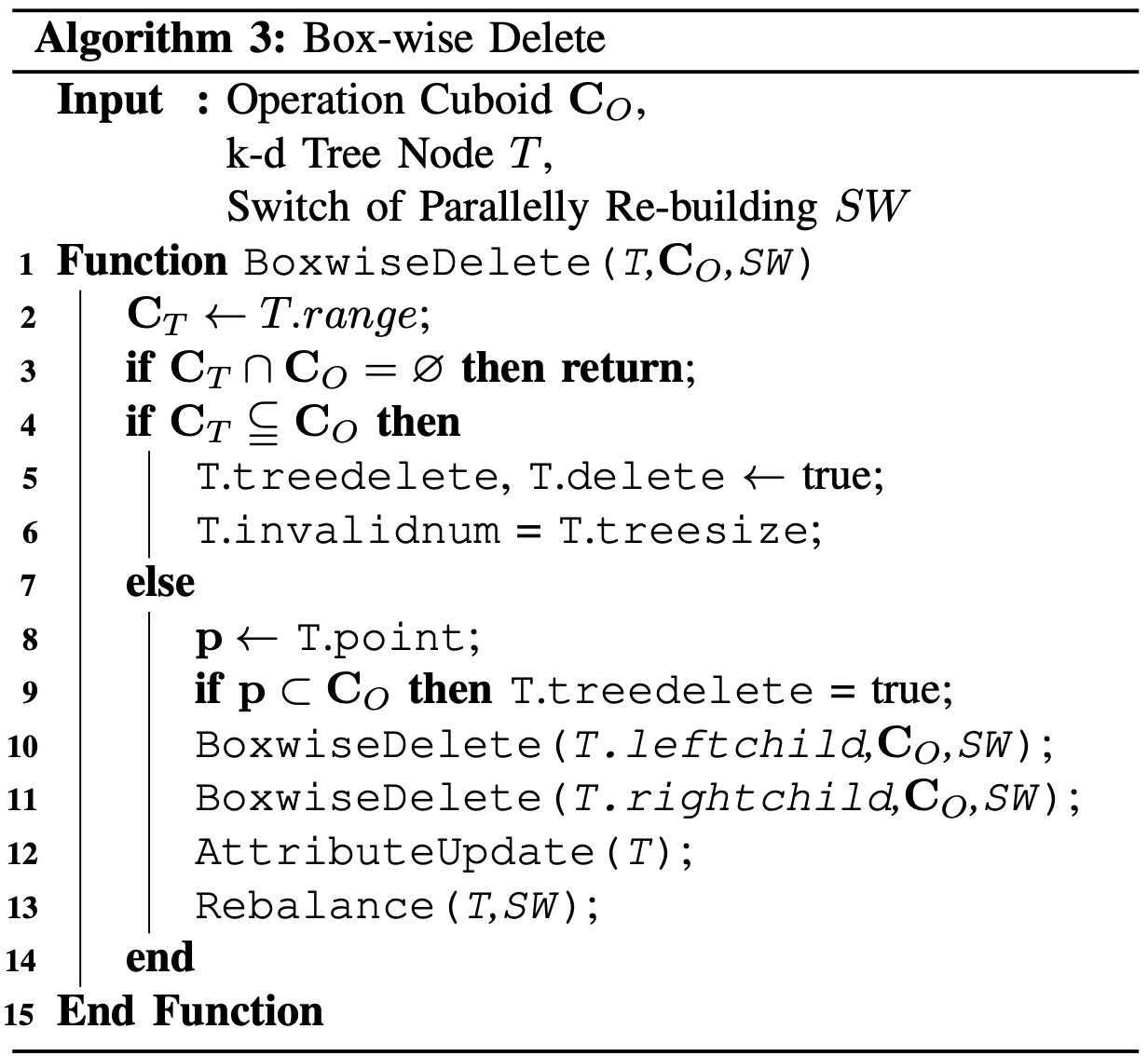
通过设置节点属性 deleted 为 true 来标记点删除,实现“懒”删除。如果根为 T T T T T T treedeleted 标记为 true。deleted 和 treedeleted 为“懒”标签。被标记为“deleted”的节点会在树的重建过程删除(参见 4.4)。
使用属性 range(长方体 C T \mathbf{C}_T C T
给定根在 T T T C O \mathbf{C}_O C O
如果 C T \mathbf{C}_T C T C O \mathbf{C}_O C O
如果 C T ⊆ C O \mathbf{C}_T \subseteq \mathbf{C}_O C T ⊆ C O deleted 和 treedeleted 标记为 true,且此时节点为根的子树的所有点被删除,因此 invalidnum 的值为树的大小;
当不满足上述两种情况,则当前点 p \mathbf{p} p C O \mathbf{C}_O C O
完成增量操作后,使用函数 AttributeUpdate 进行属性更新。该函数通过汇总当前节点的子节点的相关信息完成更新。range 的更新通过合并子节点和当前节点的信息完成。如果当前节点的子节点的 treedeleted 都为 true 且当前节点的 deleted 为 true,则当前节点的 treedeleted 设为 true。
每次增量操作后,ikd-Tree 通过重建相关子树重建树平衡。
平衡准则包含 α \alpha α α \alpha α
假设一个 ikd-Tree 的子树根为 T T T α \alpha α
S ( T . l e f t c h i l d ) < α b a l ( S ( T ) − 1 ) S ( T . r i g h t c h i l d ) < α b a l ( s ( T ) − 1 ) (17) \begin{aligned}
S(T.leftchild) &< \alpha_{bal}\left( S(T) - 1 \right)
\newline
S(T.rightchild) &< \alpha_{bal}\left( s(T) - 1 \right)
\end{aligned}
\tag{17}
S ( T . l e f t c h i l d ) < α b a l ( S ( T ) − 1 ) S ( T . r i g h t c h i l d ) < α b a l ( s ( T ) − 1 ) ( 1 7 )
其中 α b a l ∈ ( 0.5 , 1 ) \alpha_{bal} \in (0.5, 1) α b a l ∈ ( 0 . 5 , 1 ) S ( T ) S(T) S ( T ) T T T treesize。
根为 T T T α \alpha α
I ( T ) < α d e l S ( T ) (18) I(T) < \alpha_{del}S(T)
\tag{18}
I ( T ) < α d e l S ( T ) ( 1 8 )
其中 α d e l ∈ ( 0 , 1 ) \alpha_{del} \in (0, 1) α d e l ∈ ( 0 , 1 ) I ( T ) I(T) I ( T ) T T T invalidnum。
如果 ikd-Tree 的子树满足上述两个准则,则子树是平衡的;如果所有子树都是平衡的,则整棵树是平衡的。
违反任何一个准则都会触发重建过程:
α \alpha α log 1 / α b a l ( n ) \log 1/ \alpha_{bal} (n) log 1 / α b a l ( n ) n n n α \alpha α
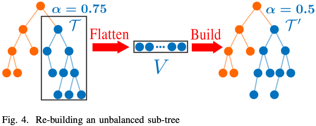
如图-4,假设在子树 T \mathcal{T} T
子树首先被展开为点列 V V V V V V
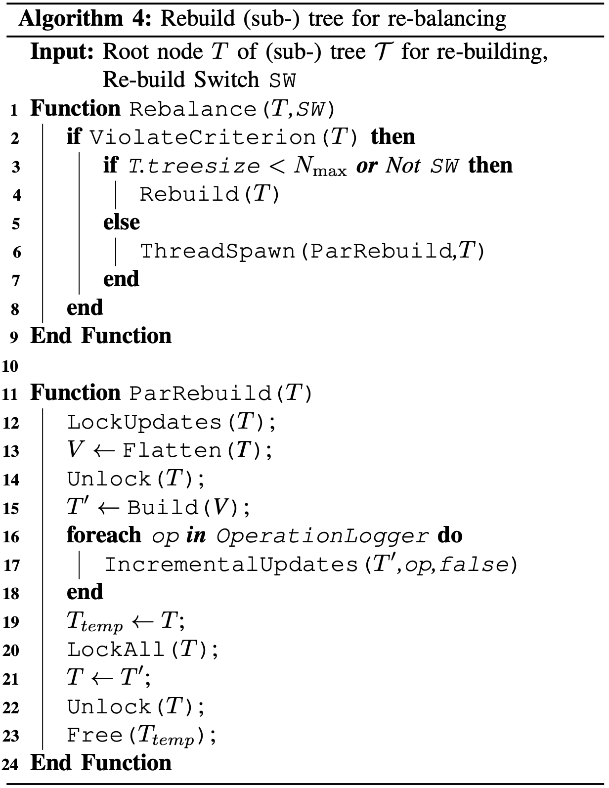
当打破平衡准则,子树大小小于阈值 N max N_{\max} N max
第二个线程的重建如 ParRebuild 函数(将第二个线程中要重建的子树表示为 T \mathcal{T} T T T T
线程锁住所有增量更新(点插入和删除),但不锁住查询(第 12 行)。
将子树 T \mathcal{T} T V V V
展开之后,原子树被解锁,以便主线程接受增量更新请求(第 14 行),这些请求将记录在 operation logger 的队列中。
一旦线程完成从 V V V T ′ \mathcal{T}^{\prime} T ′ IncrementalUpdates 再次对 T ′ \mathcal{T}^{\prime} T ′
所有请求处理完后,原子树 T \mathcal{T} T T ′ \mathcal{T}^{\prime} T ′ T T T T ′ T^{\prime} T ′
最后,释放原子树的内存(第 23 行)。
注意,LockUpdates 不会阻塞查询,查询可以在主线程中并行执行;LockAll 阻塞所有的访问,包括查询。LockUpdates 和 LockAll 通过互斥(mutex)实现。
利用节点上的范围信息,通过 [3] 中介绍的“bounds-overlap-ball”测试,加快最近邻搜索的速度。维护一个优先队列 q 来存储到目前遇到的 k k k C T \mathbf{C}_T C T d min d_{\min} d min d min d_{\min} d min q 中的最大距离,则不需要处理该节点及其子节点。
此外,在 FAST-LIO2 中,只有当近邻点在目标点周围的给定阈值内时才被视为内点用于状态估计,这为 k k k
ikd-Tree 支持多线程的 k k k
由于树上下采样的插入依赖于逐框删除和逐框搜索,因此首先讨论逐框操作。设 n n n
**定理-1:**设 ikd-Tree 上的点在空间 S x × S y × S z S_x \times S_y \times S_z S x × S y × S z C D = L x × L y × L z \mathbf{C}_D = L_x \times L_y \times L_z C D = L x × L y × L z
O ( H ( n ) ) = { O ( log n ) if Δ min ⩾ α ( 2 3 ) ( ∗ ) O ( n 1 − a − b − c ) if Δ max ⩽ 1 − α ( 1 3 ) ( ∗ ∗ ) O ( n α ( 1 3 ) − Δ min − Δ med ) if ( ∗ ) and ( ∗ ∗ ) fail and Δ med < α ( 1 3 ) − α ( 2 3 ) O ( n α ( 2 3 ) − Δ min ) otherwise. (19) O(H(n))= \begin{cases}O(\log n) & \text { if } \Delta_{\min } \geqslant \alpha\left(\frac{2}{3}\right)\left({ }^*\right) \\ O\left(n^{1-a-b-c}\right) & \text { if } \Delta_{\max } \leqslant 1-\alpha\left(\frac{1}{3}\right)(* *) \\ O\left(n^{\alpha\left(\frac{1}{3}\right)-\Delta_{\min }-\Delta_{\operatorname{med}}}\right) & \text { if }\left(^*\right) \text { and }(* *) \text { fail and } \\ & \Delta_{\text {med }}<\alpha\left(\frac{1}{3}\right)-\alpha\left(\frac{2}{3}\right) \\ O\left(n^{\alpha\left(\frac{2}{3}\right)-\Delta_{\min }}\right) & \text { otherwise. }\end{cases}
\tag{19}
O ( H ( n ) ) = ⎩ ⎪ ⎪ ⎪ ⎪ ⎪ ⎪ ⎪ ⎨ ⎪ ⎪ ⎪ ⎪ ⎪ ⎪ ⎪ ⎧ O ( log n ) O ( n 1 − a − b − c ) O ( n α ( 3 1 ) − Δ min − Δ m e d ) O ( n α ( 3 2 ) − Δ min ) if Δ min ⩾ α ( 3 2 ) ( ∗ ) if Δ max ⩽ 1 − α ( 3 1 ) ( ∗ ∗ ) if ( ∗ ) and ( ∗ ∗ ) fail and Δ med < α ( 3 1 ) − α ( 3 2 ) otherwise. ( 1 9 )
其中 a = log n S x L x , b = log n S y L y , c = log n S z L z a = \log_n \frac{S_x}{L_x}, b = \log_n \frac{S_y}{L_y}, c = \log_n \frac{S_z}{L_z} a = log n L x S x , b = log n L y S y , c = log n L z S z a , b , c ≥ 0 a, b, c \ge 0 a , b , c ≥ 0 Δ min , Δ med , Δ max \Delta_{\min}, \Delta_{\text{med}}, \Delta_{\max} Δ min , Δ med , Δ max a , b , c a, b, c a , b , c α ( u ) \alpha(u) α ( u ) u ∈ [ 0 , 1 ] , α ( 1 3 ) = 0.7162 , α ( 2 3 ) = 0.3949 u \in [0, 1], \alpha(\frac{1}{3}) = 0.7162, \alpha(\frac{2}{3}) = 0.3949 u ∈ [ 0 , 1 ] , α ( 3 1 ) = 0 . 7 1 6 2 , α ( 3 2 ) = 0 . 3 9 4 9
树上下采样的插入时间复杂度为:
**定理-2:**算法-2 的时间复杂度为 O ( log n ) O(\log n) O ( log n )
单线程重建的时间复杂度为:O ( n log n ) O(n \log n) O ( n log n )
双线程并行重建的时间复杂度为:O ( n ) O(n) O ( n )
ikd-Tree 上执行 k k k O ( log n ) O(\log n) O ( log n )
ROS,C++
迭代卡尔曼滤波器基于 IKFOM
局部地图的大小 L = 1000 m L = 1000 \text{m} L = 1 0 0 0 m
算法-2 中 l = 0.5 m l = 0.5\text{m} l = 0 . 5 m
ikd-Tree 的参数 α b a l = 0.6 , α d e l = 0.5 , N max = 1500 \alpha_{bal} = 0.6, \alpha_{del} = 0.5, N_{\max} = 1500 α b a l = 0 . 6 , α d e l = 0 . 5 , N max = 1 5 0 0
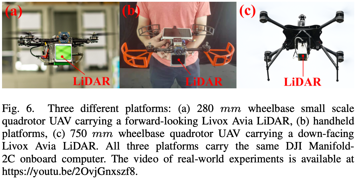
实验平台:
DJI Manifold 2-C7 {}^7 7
Khadas VIM38 {}^8 8
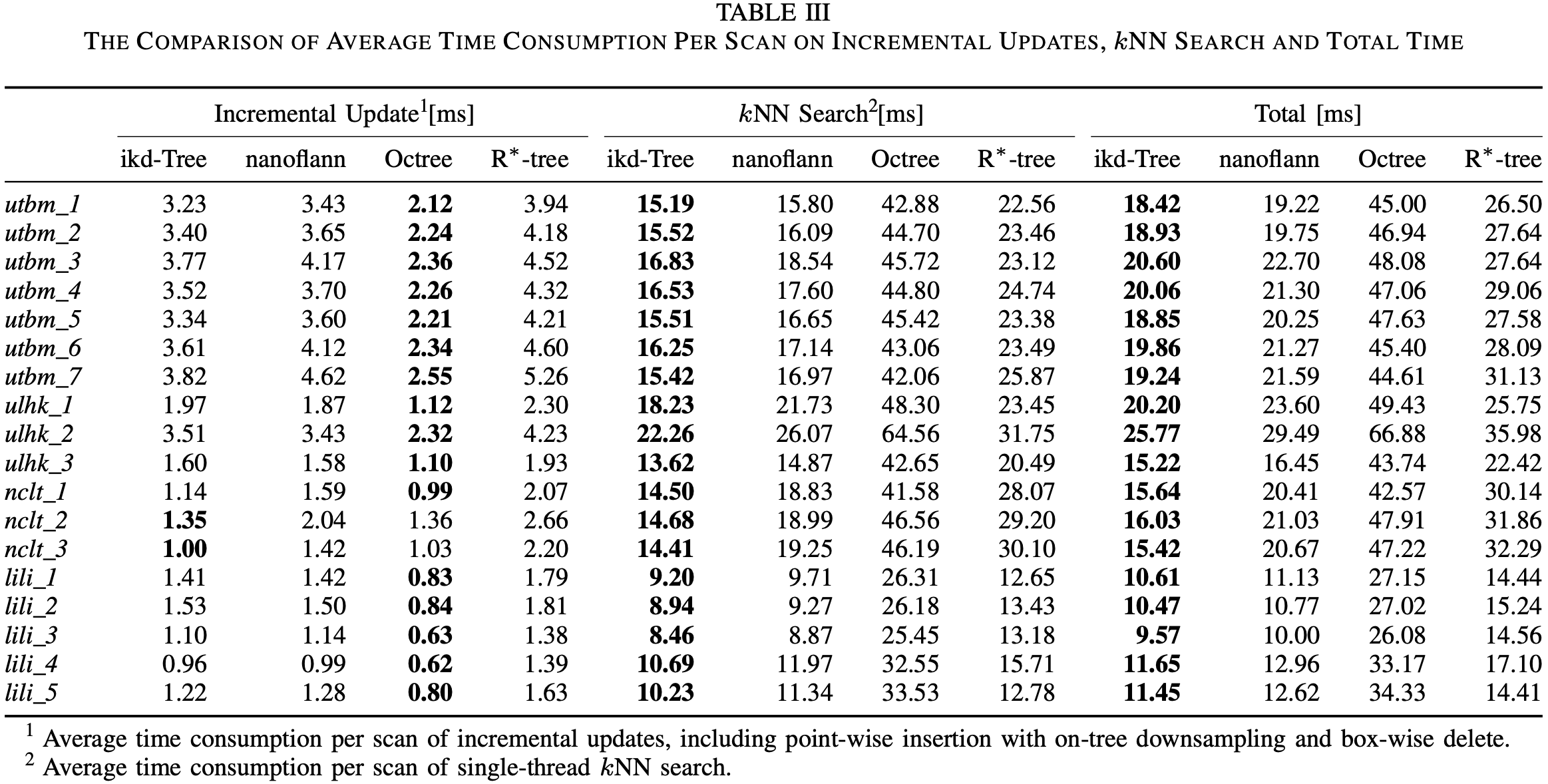
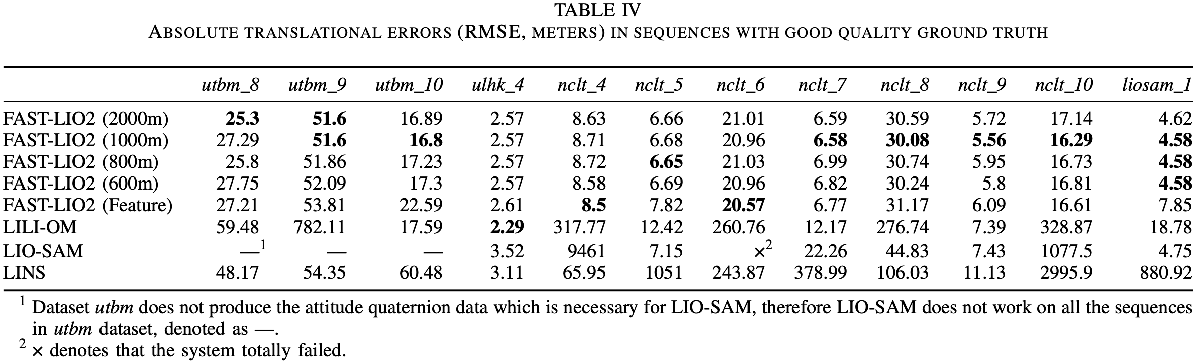
对比 L = 2000 m , 1000 m , 800 m , 600 m L = 2000\text{m}, 1000\text{m}, 800\text{m}, 600\text{m} L = 2 0 0 0 m , 1 0 0 0 m , 8 0 0 m , 6 0 0 m
[1] W. Xu and F. Zhang, “Fast-lio: A fast, robust lidar-inertial odometry package by tightly-coupled iterated kalman filter,” IEEE Robotics and Automation Letters , pp. 1–1, 2021.
[2] D. He, W. Xu, and F. Zhang, “Embedding manifold structures into kalman filters,” arXiv preprint arXiv:2102.03804 , 2021.
[3] J. H. Friedman, J. L. Bentley, and R. A. Finkel, “an algorithm for finding best matches in logarithmic expected time,” ACM Transactions on Mathematical Software (TOMS) , vol. 3, no. 3, pp. 209–226, 1977.
[4] Z. Liu and F. Zhang, “Balm: Bundle adjustment for lidar mapping,” IEEE Robotics and Automation Letters , vol. 6, no. 2, pp. 3184–3191, 2021.
设 M \mathcal{M} M n n n M = S O ( 3 ) \mathcal{M}=SO(3) M = S O ( 3 ) R n \mathbf{R}_n R n ⊞ / ⊟ \boxplus / \boxminus ⊞ / ⊟ M \mathcal{M} M R n R n Rn\mathbf{R}_n R n R n
⊞ : M × R n → M ; ⊟ : M × M → R n M ∈ S O ( 3 ) : R ⊞ r = R Exp ( r ) ; R 1 ⊟ R 2 = Log ( R 2 T R 1 ) M ∈ R n : a ⊞ b = a + b ; a ⊟ b = a − b (A-1) \begin{matrix}
\boxplus: \mathcal{M} \times \mathbb{R}^n \rightarrow \mathcal{M}; \quad \boxminus: \mathcal{M \times M} \rightarrow \mathbb{R}^n \\
\mathcal{M} \in SO(3): \mathbf{R \boxplus r = R} \operatorname{Exp}(\mathbf{r}); \quad \mathbf{R}_1 \boxminus \mathbf{R}_2 = \operatorname{Log}(\mathbf{R}_2^T \mathbf{R}_1) \\
\mathcal{M} \in \mathbb{R}^n: \mathbf{a \boxplus b} = \mathbf{a} + \mathbf{b}; \quad \mathbf{a \boxminus b} = \mathbf{a} - \mathbf{b}
\end{matrix}
\tag{A-1}
⊞ : M × R n → M ; ⊟ : M × M → R n M ∈ S O ( 3 ) : R ⊞ r = R E x p ( r ) ; R 1 ⊟ R 2 = L o g ( R 2 T R 1 ) M ∈ R n : a ⊞ b = a + b ; a ⊟ b = a − b ( A - 1 )
对于复合流形 M ∈ S O ( 3 ) × R n \mathcal{M} \in SO(3) \times \mathbb{R}^n M ∈ S O ( 3 ) × R n
[ R a ] ⊞ [ r b ] = [ R ⊞ r a + b ] , [ R 1 a ] ⊟ [ R 2 b ] = [ R 1 ⊟ R 1 a − b ] (A-2) \left[
\begin{matrix}
\mathbf{R} \\
\mathbf{a}
\end{matrix}
\right]
\boxplus
\left[
\begin{matrix}
\mathbf{r} \\
\mathbf{b}
\end{matrix}
\right]
=
\left[
\begin{matrix}
\mathbf{R \boxplus r} \\
\mathbf{a + b}
\end{matrix}
\right]
, \quad
\left[
\begin{matrix}
\mathbf{R}_1 \\
\mathbf{a}
\end{matrix}
\right]
\boxminus
\left[
\begin{matrix}
\mathbf{R}_2 \\
\mathbf{b}
\end{matrix}
\right]
=
\left[
\begin{matrix}
\mathbf{R}_1 \boxminus \mathbf{R}_1 \\
\mathbf{a} - \mathbf{b}
\end{matrix}
\right]
\tag{A-2}
[ R a ] ⊞ [ r b ] = [ R ⊞ r a + b ] , [ R 1 a ] ⊟ [ R 2 b ] = [ R 1 ⊟ R 1 a − b ] ( A - 2 )
易验证:
( x ⊞ u ) ⊟ x = u , x ⊞ ( y ⊟ x ) = y ; ∀ x , y ∈ M , u ∈ R n (A-3) (\mathbf{x} \boxplus \mathbf{u}) \boxminus \mathbf{x} = \mathbf{u}, \mathbf{x} \boxplus (\mathbf{y} \boxminus \mathbf{x}) = \mathbf{y}; \forall \mathbf{x}, \mathbf{y} \in \mathcal{M}, \mathbf{u} \in \mathbb{R}^n
\tag{A-3}
( x ⊞ u ) ⊟ x = u , x ⊞ ( y ⊟ x ) = y ; ∀ x , y ∈ M , u ∈ R n ( A - 3 )
A ( ⋅ ) − 1 \mathbf{A}(\cdot)^{-1} A ( ⋅ ) − 1 对 A ( ⋅ ) − 1 \mathbf{A}(\cdot)^{-1} A ( ⋅ ) − 1
A ( u ) − 1 = I − 1 2 ⌊ u ⌋ ∧ + ( 1 − α ( ∥ u ∥ ) ) ⌊ u ⌋ Λ 2 ∥ u ∥ 2 α ( m ) = m 2 cot ( m 2 ) = m 2 cos ( m / 2 ) sin ( m / 2 ) (B-1) \begin{aligned}
\mathbf{A}(\mathbf{u})^{-1} & =\mathbf{I}-\frac{1}{2}\lfloor\mathbf{u}\rfloor_{\wedge}+(1-\boldsymbol{\alpha}(\|\mathbf{u}\|)) \frac{\lfloor\mathbf{u}\rfloor_{\Lambda}^2}{\|\mathbf{u}\|^2} \\
\alpha(\mathrm{m}) & =\frac{\mathrm{m}}{2} \cot \left(\frac{\mathrm{m}}{2}\right)=\frac{\mathrm{m}}{2} \frac{\cos (\mathrm{m} / 2)}{\sin (\mathrm{m} / 2)}
\end{aligned}
\tag{B-1}
A ( u ) − 1 α ( m ) = I − 2 1 ⌊ u ⌋ ∧ + ( 1 − α ( ∥ u ∥ ) ) ∥ u ∥ 2 ⌊ u ⌋ Λ 2 = 2 m cot ( 2 m ) = 2 m sin ( m / 2 ) cos ( m / 2 ) ( B - 1 )